
Mathematical Foundations of Machine Learning
Mathematical Foundations of Machine Learning
Machine learning might seem like magic, but it's built on solid mathematical foundations. Understanding these concepts isn't just academic—it's the key to building better models, debugging problems, and pushing the field forward.
Why Mathematics Matters in ML
Before diving into specific topics, let's understand why mathematics is crucial:
- Model Design: Math helps us understand what models can and cannot do
- Optimization: We need calculus to train models efficiently
- Uncertainty: Probability theory helps us handle noisy, incomplete data
- Dimensionality: Linear algebra lets us work with high-dimensional data
Linear Algebra: The Language of Data
Linear algebra is everywhere in machine learning. From representing data as vectors to understanding neural network transformations, it's fundamental.
Vectors and Matrices
import numpy as np

# Data as vectors
x = np.array([1.5, 2.3, 0.8])  # A data point
X = np.array([[1.5, 2.3, 0.8],  # Dataset as matrix
              [2.1, 1.9, 1.2],
              [0.9, 3.1, 0.5]])

# Matrix operations
W = np.array([[0.5, 0.3],     # Weight matrix
              [0.2, 0.8],
              [0.1, 0.4]])

# Linear transformation
output = X @ W  # Matrix multiplication
print(f"Transformed data shape: {output.shape}")
Eigenvalues and Eigenvectors
These are crucial for understanding Principal Component Analysis (PCA):
# Compute covariance matrix
cov_matrix = np.cov(X.T)

# Find eigenvalues and eigenvectors
eigenvalues, eigenvectors = np.linalg.eig(cov_matrix)

print(f"Eigenvalues: {eigenvalues}")
print(f"Principal component: {eigenvectors[:, 0]}")
Key Linear Algebra Concepts for ML
- Matrix Multiplication: Foundation of neural networks
- Rank and Span: Understanding data dimensionality
- Norms: Measuring distances and regularization
- Decompositions: SVD, eigendecomposition for dimensionality reduction
Calculus: The Engine of Optimization
Machine learning models learn by optimizing objective functions. Calculus makes this possible.
Gradients and Derivatives
import matplotlib.pyplot as plt

def quadratic_function(x):
    return x**2 + 2*x + 1

def gradient(x):
    return 2*x + 2

# Gradient descent example
x = 5.0  # Starting point
learning_rate = 0.1
history = [x]

for i in range(20):
    grad = gradient(x)
    x = x - learning_rate * grad
    history.append(x)

print(f"Final x: {x:.4f}")
print(f"Final function value: {quadratic_function(x):.4f}")
Chain Rule and Backpropagation
The chain rule is the mathematical foundation of backpropagation:
# Simple example of chain rule in action
def sigmoid(x):
    return 1 / (1 + np.exp(-x))

def sigmoid_derivative(x):
    s = sigmoid(x)
    return s * (1 - s)

# Forward pass
x = 2.0
w = 0.5
z = w * x
a = sigmoid(z)

# Backward pass (chain rule)
dL_da = 2 * (a - 1)  # Assuming squared loss
da_dz = sigmoid_derivative(z)
dz_dw = x

dL_dw = dL_da * da_dz * dz_dw
print(f"Gradient w.r.t. weight: {dL_dw:.4f}")
Multivariable Calculus
Real ML problems involve functions of many variables:
# Gradient of a multivariable function
def multivar_function(w):
    x, y = w[0], w[1]
    return x**2 + 2*y**2 + x*y

def compute_gradient(w):
    x, y = w[0], w[1]
    return np.array([2*x + y, 4*y + x])

# Gradient descent for multivariable function
w = np.array([3.0, 2.0])
learning_rate = 0.1

for i in range(50):
    grad = compute_gradient(w)
    w = w - learning_rate * grad

print(f"Optimized weights: {w}")
Probability: Handling Uncertainty
Machine learning deals with uncertainty everywhere—noisy data, model uncertainty, prediction confidence.
Probability Distributions
import scipy.stats as stats

# Normal distribution - ubiquitous in ML
mu, sigma = 0, 1
x = np.linspace(-4, 4, 100)
pdf = stats.norm.pdf(x, mu, sigma)

plt.figure(figsize=(10, 6))
plt.subplot(1, 2, 1)
plt.plot(x, pdf, 'b-', label=f'Normal(μ={mu}, σ={sigma})')
plt.title('Probability Density Function')
plt.legend()

# Bernoulli distribution - for binary classification
p = 0.7
outcomes = stats.bernoulli.rvs(p, size=1000)
plt.subplot(1, 2, 2)
plt.hist(outcomes, bins=2, density=True, alpha=0.7)
plt.title(f'Bernoulli Distribution (p={p})')
plt.show()
Bayes' Theorem
The foundation of Bayesian machine learning:
# Bayesian inference example
def bayesian_update(prior, likelihood, evidence):
    posterior = (likelihood * prior) / evidence
    return posterior

# Example: coin flip inference
prior_fair = 0.5  # Prior belief coin is fair
likelihood_10_heads = 0.5**10  # Likelihood of 10 heads if fair
likelihood_10_heads_biased = 0.9**10  # If biased towards heads

# Evidence (total probability)
evidence = likelihood_10_heads * prior_fair + likelihood_10_heads_biased * (1 - prior_fair)

posterior_fair = bayesian_update(prior_fair, likelihood_10_heads, evidence)
print(f"Posterior probability coin is fair: {posterior_fair:.4f}")
Maximum Likelihood Estimation
# MLE for normal distribution
def log_likelihood_normal(data, mu, sigma):
    n = len(data)
    ll = -n/2 * np.log(2 * np.pi * sigma**2)
    ll -= np.sum((data - mu)**2) / (2 * sigma**2)
    return ll

# Generate sample data
np.random.seed(42)
true_mu, true_sigma = 3.0, 1.5
data = np.random.normal(true_mu, true_sigma, 100)

# MLE estimates
mle_mu = np.mean(data)
mle_sigma = np.std(data, ddof=0)

print(f"True parameters: μ={true_mu}, σ={true_sigma}")
print(f"MLE estimates: μ={mle_mu:.3f}, σ={mle_sigma:.3f}")
Information Theory
Information theory provides tools for understanding data compression, feature selection, and model complexity.
Entropy
def entropy(probabilities):
    """Calculate Shannon entropy"""
    p = np.array(probabilities)
    p = p[p > 0]  # Remove zero probabilities
    return -np.sum(p * np.log2(p))

# Example: entropy of coin flips
fair_coin = [0.5, 0.5]
biased_coin = [0.9, 0.1]

print(f"Fair coin entropy: {entropy(fair_coin):.3f} bits")
print(f"Biased coin entropy: {entropy(biased_coin):.3f} bits")
Mutual Information
from sklearn.metrics import mutual_info_score

# Generate correlated data
x = np.random.randint(0, 3, 1000)
y = (x + np.random.randint(0, 2, 1000)) % 3  # y depends on x

mi = mutual_info_score(x, y)
print(f"Mutual information between x and y: {mi:.3f}")
Putting It All Together
Here's how these mathematical concepts work together in a simple neural network:
class SimpleNeuralNetwork:
    def __init__(self, input_size, hidden_size, output_size):
        # Linear algebra: weight matrices
        self.W1 = np.random.randn(input_size, hidden_size) * 0.1
        self.W2 = np.random.randn(hidden_size, output_size) * 0.1
        self.b1 = np.zeros((1, hidden_size))
        self.b2 = np.zeros((1, output_size))

    def forward(self, X):
        # Linear algebra: matrix operations
        self.z1 = X @ self.W1 + self.b1
        self.a1 = sigmoid(self.z1)  # Calculus: derivative needed for backprop
        self.z2 = self.a1 @ self.W2 + self.b2
        self.a2 = sigmoid(self.z2)
        return self.a2

    def backward(self, X, y, output):
        m = X.shape[0]

        # Calculus: chain rule for gradients
        dz2 = output - y
        dW2 = (1/m) * self.a1.T @ dz2
        db2 = (1/m) * np.sum(dz2, axis=0, keepdims=True)

        da1 = dz2 @ self.W2.T
        dz1 = da1 * sigmoid_derivative(self.z1)
        dW1 = (1/m) * X.T @ dz1
        db1 = (1/m) * np.sum(dz1, axis=0, keepdims=True)

        return dW1, db1, dW2, db2

    def train(self, X, y, epochs, learning_rate):
        for epoch in range(epochs):
            # Forward pass
            output = self.forward(X)

            # Probability: compute loss
            loss = np.mean((output - y)**2)

            # Backward pass
            dW1, db1, dW2, db2 = self.backward(X, y, output)

            # Calculus: gradient descent update
            self.W1 -= learning_rate * dW1
            self.b1 -= learning_rate * db1
            self.W2 -= learning_rate * dW2
            self.b2 -= learning_rate * db2

            if epoch % 100 == 0:
                print(f"Epoch {epoch}, Loss: {loss:.4f}")

# Example usage
X = np.random.randn(100, 2)
y = (X[:, 0] + X[:, 1] > 0).astype(int).reshape(-1, 1)

nn = SimpleNeuralNetwork(2, 4, 1)
nn.train(X, y, epochs=1000, learning_rate=0.1)
Conclusion
Mathematics isn't just the foundation of machine learning—it's the key to understanding, debugging, and improving your models. While libraries abstract away many details, understanding the underlying math helps you:
- Choose appropriate models for your problems
- Debug when things go wrong
- Optimize performance and efficiency
- Contribute to advancing the field
The journey to mathematical mastery is gradual, but every concept you understand makes you a better machine learning practitioner.
Next up: Check out my post on Bayesian Methods in Machine Learning to dive deeper into probabilistic approaches.
Related Posts
More content from the Mathematics category and similar topics
A simple explaination of projectiong points onto a hyperspace.
Shared topics:

Learn the fundamentals of Functional Data Analysis and how to implement key techniques using R.
Shared topics:
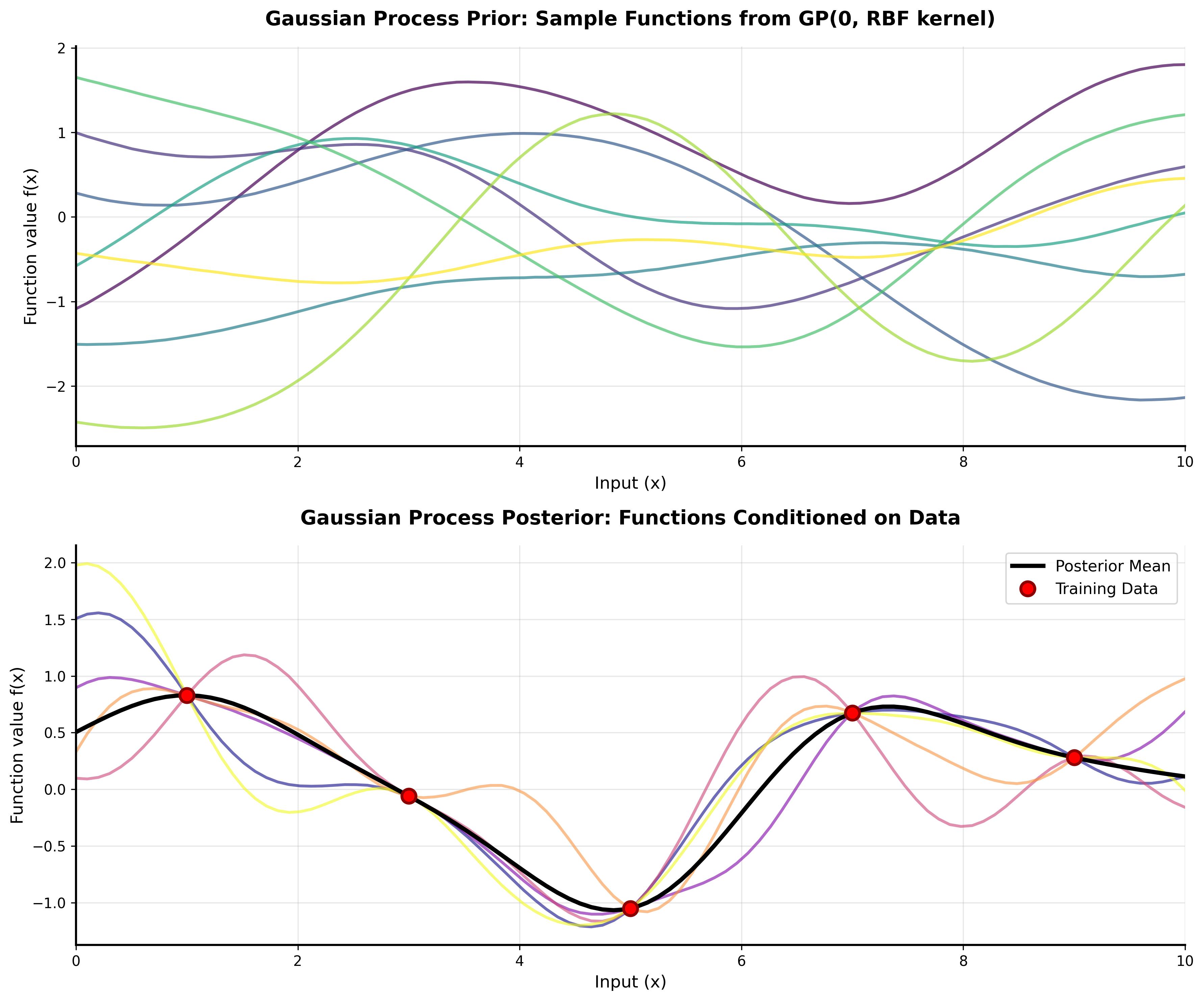
A comprehensive tutorial on understanding Gaussian Processes with interactive visualizations and practical examples.
Shared topics: