
Projection onto Hyperspace
Projection onto Hyperplane
Projections play an important role in Linear algebra, optimization, and machine learning. Some time we are interested in projecting points onto a lower dimensional space, or say, a general subspace of a higher dimensinal space.
In this note, we explain how to derive the projection formula of a point onto a hyperspace. The derivation works the same when the hyperspace is replaced by a plane or a line.
0. Notations
We consider vectors in and use the inner product notation for vectors . The norm of a vector is denoted by . We denote by the zero vecor of . We also use the notation to mean that and are orthogonal, i.e. .
1. Hyperspace
Let be two vectors. The set defined by is called a hyperplane of spanned by passing through by .
Additionally, the vector is orthogonal to , i.e. In fact, if , then and , which implies that .
Fact 1 : Any vctor orthogonal to is a multiple of , i.e. for some .
Proof: we already know that for all . So, is any multiple of . Assume , i.e for all . Now, for a fixed , we also have . Hence,
this is true for all . This means that has to be zero, i.e. .
2. Projection onto
The prblem consists of projecting onto , that is, finding such that and is orthogonal to .
Claim : The projection of onto is given by
Proof: We know the following :
- , i.e is orthogonal to .
From fact 1, we write for some , that is
Because, , we must have , according to the definition of . Using above, we have
Therefore,
Inserting this into , we obtain
Which proves our claim. It is the projection of onto the hyperplane .
3. Applications
As we have alrady mentioned earlier, projections are widely used whether in science or in engineering. To illustration this statement, we will consider some xamples of algorithms or techniques that use (the idea of ) orthogonal projections.
Our first examples are from the field of (Randomized) Linear Algebrae and Optimization.
1. The Karczmarz method
The Karczmarz method is an iterative methods intensively for solving overdetermied systems of linear equations. The method, named after its initiator, the Polish mathenatician Stefan Karczmarz, has gained popularity in the optimization community because of its simplicity and effectictiveness in solving large-scale linear systems, like those arise in machine learning (e.g. linear regression). For a broad litterature review,see these papers 1, 2, and 3.
Consider the system of linear equations where is a matrix with equations and variables, and is a vector of constants. That is, we have the system
We assume the the system is consistent, i.e. it exists such that and . The (classic) Karczmarz Method method iteratively projects an initial guess onto the hyperplane for . That is, at an iteration , the KM select a row of and computes the projection of onto the hyperspace spanned by the row , i.e. , to obtain
We recogize that is is the same projection formula derived above.
What the (classic) KM methds does is, at iteration k, to project the current iterate onto the hyperplane spanned by the rows of , i.e , and repeates this process untill a stopping condition is met.
The full algorithm is as follows:
Procedure Karczmarz(A, b, x₀, max_iter)
Input: Matrix A ∈ ℝ^{m×n}, vector b ∈ ℝ^m, initial guess x₀ ∈ ℝ^n, maximum iterations max_iter
1. Set x = x₀
2. For k = 1 to max_iter do:
    a. Select i_k ∈ {1, ..., m}, s.t i_k = k mod m +1
    b. Let a_i be the i-th row of A
    c. Let b_i be the i-th entry of b
    d. Update:
        x ← x + [(b_i - ⟨a_i, x⟩) / ⟨a_i, a_i⟩] * a_i
3. Return x
For the python implementation, we can use the following code snippet:
def karczmarz(A, b, x0, max_iter=1000):
    m, n = A.shape
    x = x0.copy()
    for k in range(max_iter):
        i_k = k % m  # Cyclically select a row
        a_i = A[i, :]
        b_i = b[i]
        # Project onto the hyperplane defined by a_i
        x += (b_i - np.dot(a_i, x)) / np.dot(a_i, a_i) * a_i
    return x
Analytical Example: Consider the consistent overdetermined system
whose exact solution is
(since , , and ).
Kaczmarz update
Given row and scalar , one step is the orthogonal projection
This enforces .
We start from and use cyclic rows .
**Iterations (arithmetic operations): **
-
, row 1: ,
-
, row 2: ,
-
, row 3: ,
-
, row 1:
-
, row 2:
-
, row 3:
Several papers have showed the converges of the KM algorithm under various conditions. One of the issue of the (classical) KM is that it can be slow to converge, especially for large systems: it is shown in the litterature that its converegence rate depends on the row order of the matruix .
To address this issue, Strohmer et al [1] introduced the Randomized Karczmarz Method (RKM), which randomly selects a row of at each iteration. They have shown randomization helps to improve the convergence rate and robustness of the method, especially for large-scale problems.
The RKM algorithm is as follows:
Procedure Randomized Karczmarz(A, b, x₀, max_iter)
Input: Matrix A ∈ ℝ^{m×n}, vector b ∈ ℝ^m, initial guess x₀ ∈ ℝ^n, maximum iterations max_iter
1. Set x = x₀
2. For k = 1 to max_iter do:
    a. Randomly select i_k ∈ {1, ..., m} with probability proportional p_i = ||a_i ||/||A||_F^2
    b. Let a_i be the i-th row of A
    c. Let b_i be the i-th entry of b
    d. Update:
        x ← x + [(b_i - ⟨a_i, x⟩) / ⟨a_i, a_i⟩] * a_i
3. Return x
Its python implementation is as follows:
def randomized_karczmarz(A, b, x0, max_iter=1000):
    m, n = A.shape
    x = x0.copy()
    for k in range(max_iter):
        i_k = np.random.choice(m, p=np.linalg.norm(A, axis=1) / np.linalg.norm(A, ord='fro')**2)
        a_i = A[i_k, :]
        b_i = b[i_k]
        # Project onto the hyperplane defined by a_i
        x += (b_i - np.dot(a_i, x)) / np.dot(a_i,a_i) *a_i
    return x
To illustration the usefullness of projctions, we are going to to give a detailled proof of the main result of the paper by Strohmer et al [1]. For that, we need to precise some notations and definitions.
2. Least Squares Regression
Related Posts
More content from the Mathematics category and similar topics
A deep dive into the essential mathematical concepts behind modern machine learning algorithms.
Shared topics:

Learn the fundamentals of Functional Data Analysis and how to implement key techniques using R.
Shared topics:
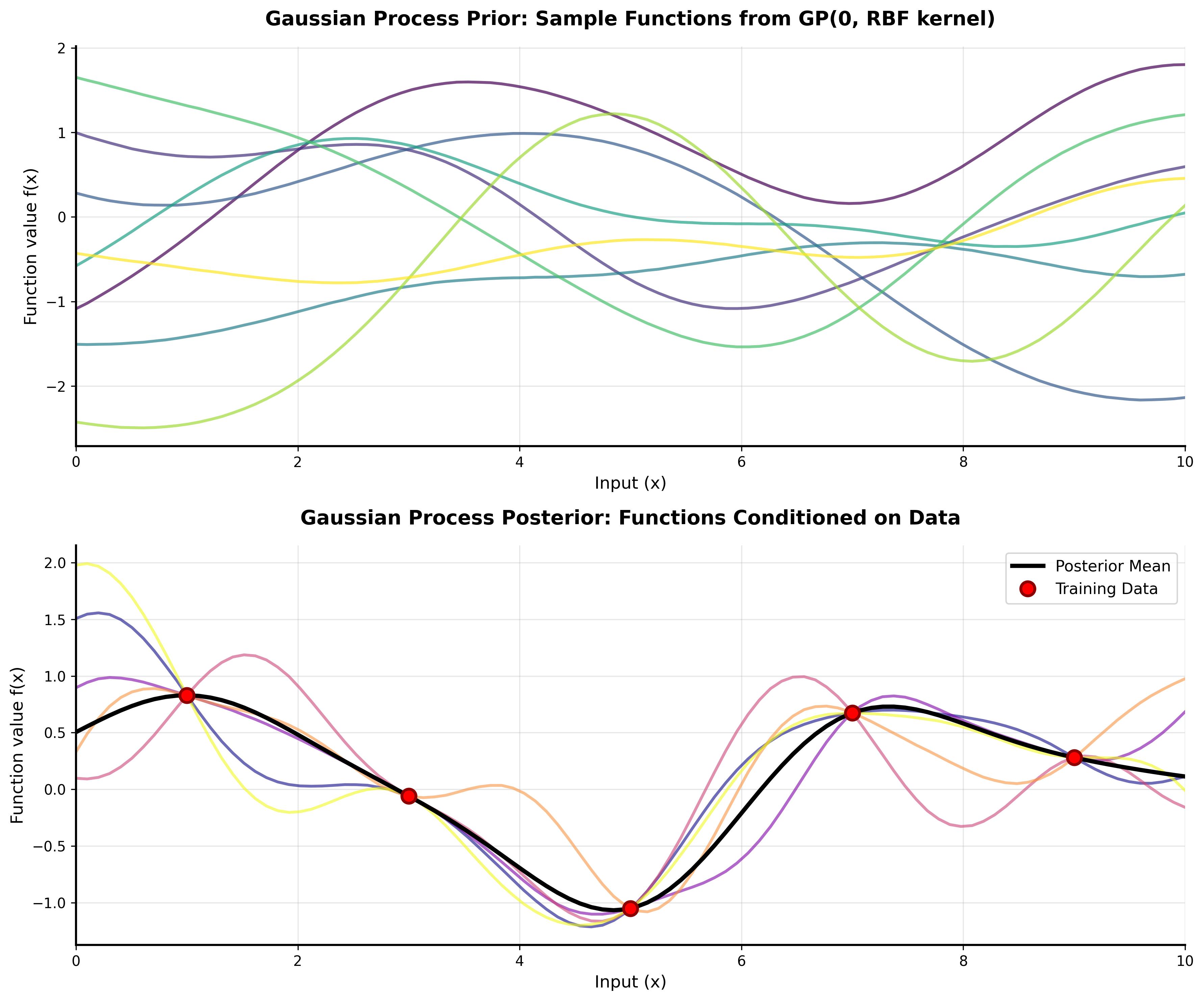
A comprehensive tutorial on understanding Gaussian Processes with interactive visualizations and practical examples.
Shared topics: