Gaussian Processes Explained: A Visual Introduction
Gaussian Processes Explained: A Visual Introduction
Gaussian Processes (GPs) are among the most elegant and powerful tools in machine learning and statistics. They provide a principled, probabilistic approach to regression and classification that naturally handles uncertainty quantification.
What are Gaussian Processes?
A Gaussian Process is a collection of random variables, any finite number of which have a joint Gaussian distribution. In the context of machine learning, we use GPs to define distributions over functions.
Mathematical Foundation
Formally, a Gaussian Process is completely specified by its mean function and covariance function :
Where:
- is the mean function
- is the covariance function
Example :
Example of Matrix rendering:
Test Latex code for the Simpson method:
Matrix Notation
For a finite set of input points , we can represent the Gaussian Process in matrix form:
Where:
- is the vector of function values
- is the mean vector
- is the covariance matrix with entries
The covariance matrix has the form:
For predictions at test points , the joint distribution is:
Where:
- is the cross-covariance matrix between training and test points
- is the covariance matrix of test points
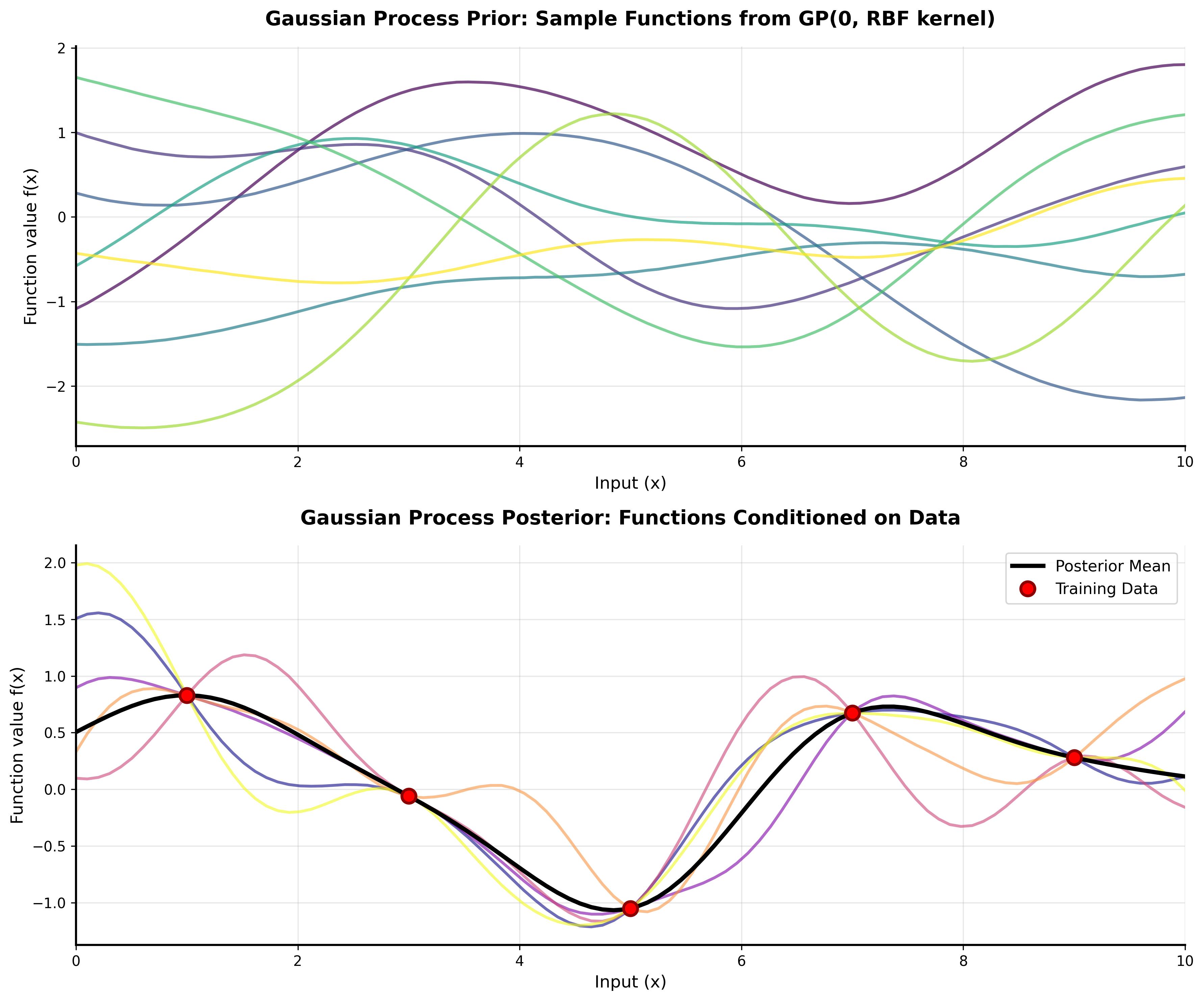
 Figure 1: A Gaussian Process with RBF kernel showing the mean prediction (blue line) and uncertainty bands (shaded area). The red dots represent training data points.
Key Properties
- Flexible non-parametric model: GPs don't assume a fixed functional form
- Uncertainty quantification: They provide error bars on predictions
- Kernel-based: The choice of kernel determines the properties of functions we're modeling
Common Kernels
The choice of kernel function is crucial as it encodes our assumptions about the function we're modeling. Here are some popular kernels:
 Figure 2: Comparison of common GP kernels showing their covariance functions.
RBF (Radial Basis Function) Kernel
import numpy as np

def rbf_kernel(x1, x2, length_scale=1.0, variance=1.0):
    """
    RBF kernel function
    """
    sqdist = np.sum(x1**2, 1).reshape(-1, 1) + np.sum(x2**2, 1) - 2 * np.dot(x1, x2.T)
    return variance * np.exp(-0.5 / length_scale**2 * sqdist)
Matérn Kernel
The Matérn kernel is a generalization of the RBF kernel and is particularly useful for modeling functions that are not infinitely differentiable.
Implementation Example
Here's a simple implementation of Gaussian Process regression:
import numpy as np
import matplotlib.pyplot as plt
from scipy.linalg import solve_triangular, cholesky
from scipy.optimize import minimize

class GaussianProcessRegressor:
    def __init__(self, kernel, noise_variance=1e-6):
        self.kernel = kernel
        self.noise_variance = noise_variance

    def fit(self, X, y):
        self.X_train = X
        self.y_train = y

        # Compute kernel matrix
        K = self.kernel(X, X)
        K += self.noise_variance * np.eye(len(X))

        # Cholesky decomposition for numerical stability
        self.L = cholesky(K, lower=True)
        self.alpha = solve_triangular(self.L, y, lower=True)

    def predict(self, X_test, return_std=False):
        K_star = self.kernel(self.X_train, X_test)
        mu = K_star.T @ solve_triangular(self.L, self.alpha, lower=True)

        if return_std:
            K_star_star = self.kernel(X_test, X_test)
            v = solve_triangular(self.L, K_star, lower=True)
            var = np.diag(K_star_star) - np.sum(v**2, axis=0)
            return mu, np.sqrt(var)

        return mu

# Example usage
X_train = np.array([[1], [3], [5], [6], [7], [8]])
y_train = np.array([1, 3, 5, 6, 7, 8]) + 0.1 * np.random.randn(6)

# Create and fit the model
gp = GaussianProcessRegressor(lambda x1, x2: rbf_kernel(x1, x2, length_scale=1.0))
gp.fit(X_train, y_train)

# Make predictions
X_test = np.linspace(0, 10, 100).reshape(-1, 1)
mu, std = gp.predict(X_test, return_std=True)

# Plot results
plt.figure(figsize=(10, 6))
plt.plot(X_train, y_train, 'ro', label='Training data')
plt.plot(X_test, mu, 'b-', label='Mean prediction')
plt.fill_between(X_test.ravel(), mu - 2*std, mu + 2*std, alpha=0.3, label='95% confidence')
plt.legend()
plt.title('Gaussian Process Regression')
plt.show()
Applications
Gaussian Processes are particularly useful in:
- Bayesian Optimization: Finding global optima of expensive black-box functions
- Time Series Modeling: Capturing temporal dependencies with appropriate kernels
- Spatial Statistics: Kriging and geostatistics
- Active Learning: Selecting informative data points based on uncertainty
Advantages and Limitations
Advantages
- Probabilistic predictions with uncertainty quantification
- No need to specify functional form a priori
- Works well with small datasets
- Principled hyperparameter learning via marginal likelihood
Limitations
- Computational complexity O(n³) for training
- Memory requirements O(n²)
- Choice of kernel can be challenging
- May struggle with high-dimensional inputs
Conclusion
Gaussian Processes provide a powerful and elegant framework for regression and classification. Their ability to quantify uncertainty makes them particularly valuable in scientific applications and decision-making under uncertainty.
The key to successful GP modeling lies in choosing appropriate kernels and properly handling computational considerations for larger datasets through techniques like sparse GPs or inducing points.
Want to learn more? Check out my other posts on Bayesian Methods and Mathematical Foundations.
Related Posts
More content from the Machine Learning category and similar topics

A comprehensive tutorial on understanding Gaussian Processes with interactive visualizations and practical examples.
Shared topics:
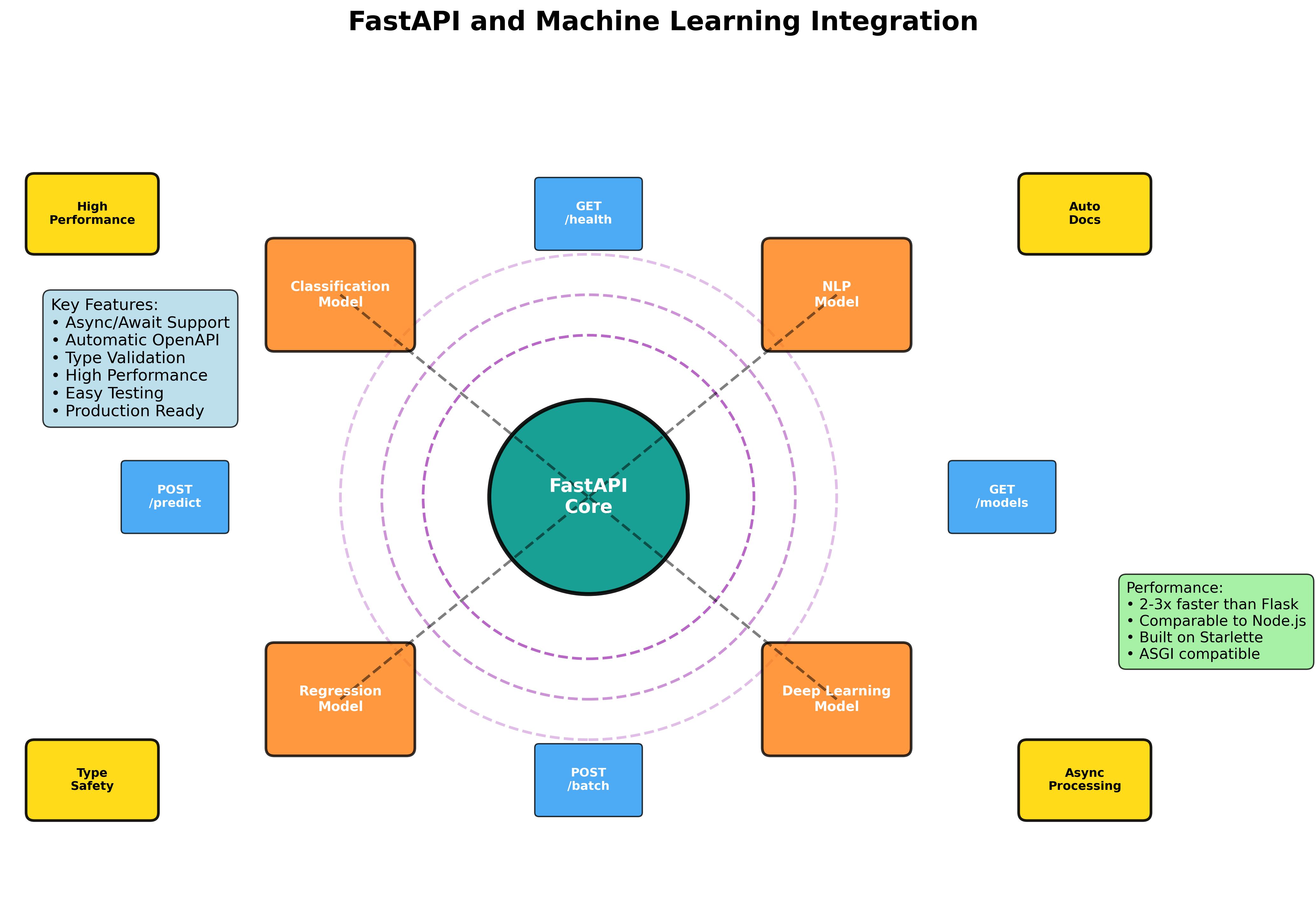
Master the art of building production-ready machine learning APIs with FastAPI. From basic model serving to advanced async processing and containerized deployment.
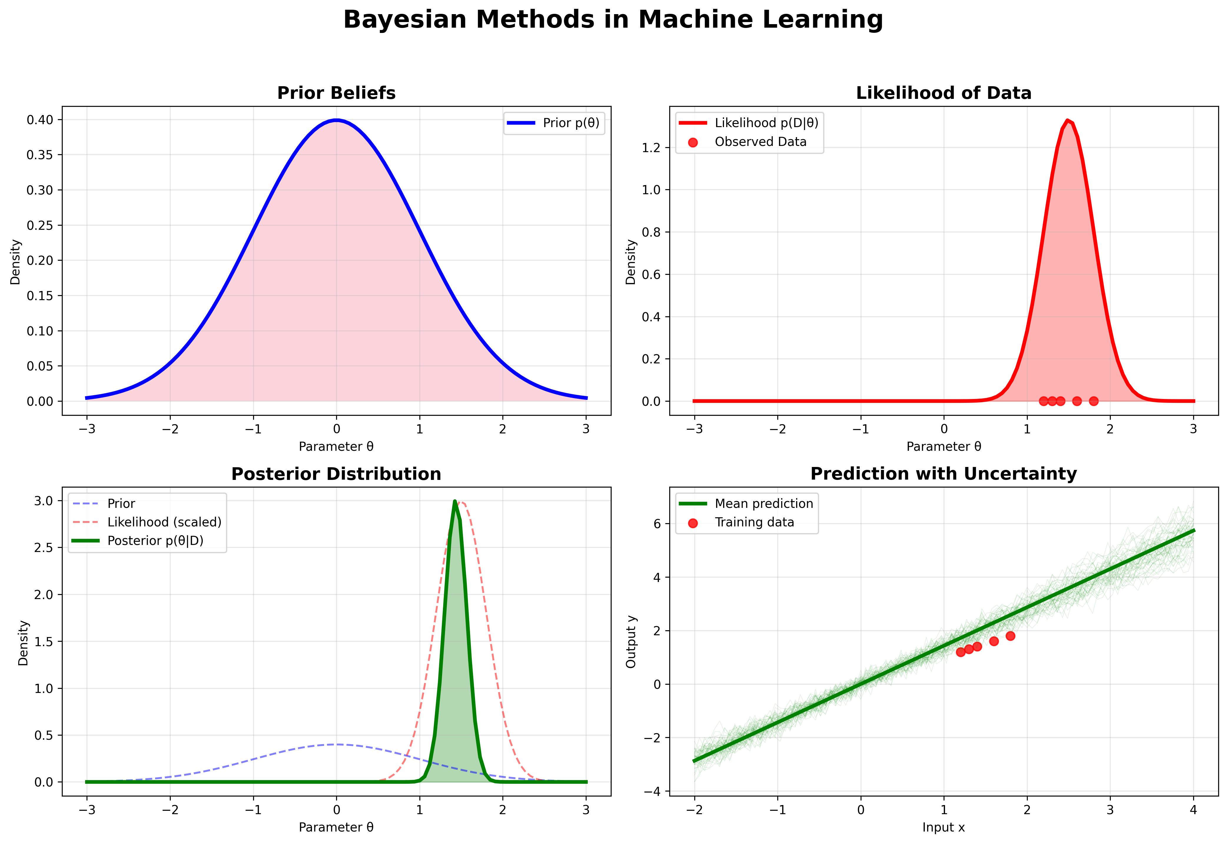
Explore the fundamental principles of Bayesian machine learning, from basic probability theory to advanced applications in modern AI systems.