Bayesian Methods in Machine Learning: A Complete Guide
Bayesian Methods in Machine Learning: A Complete Guide
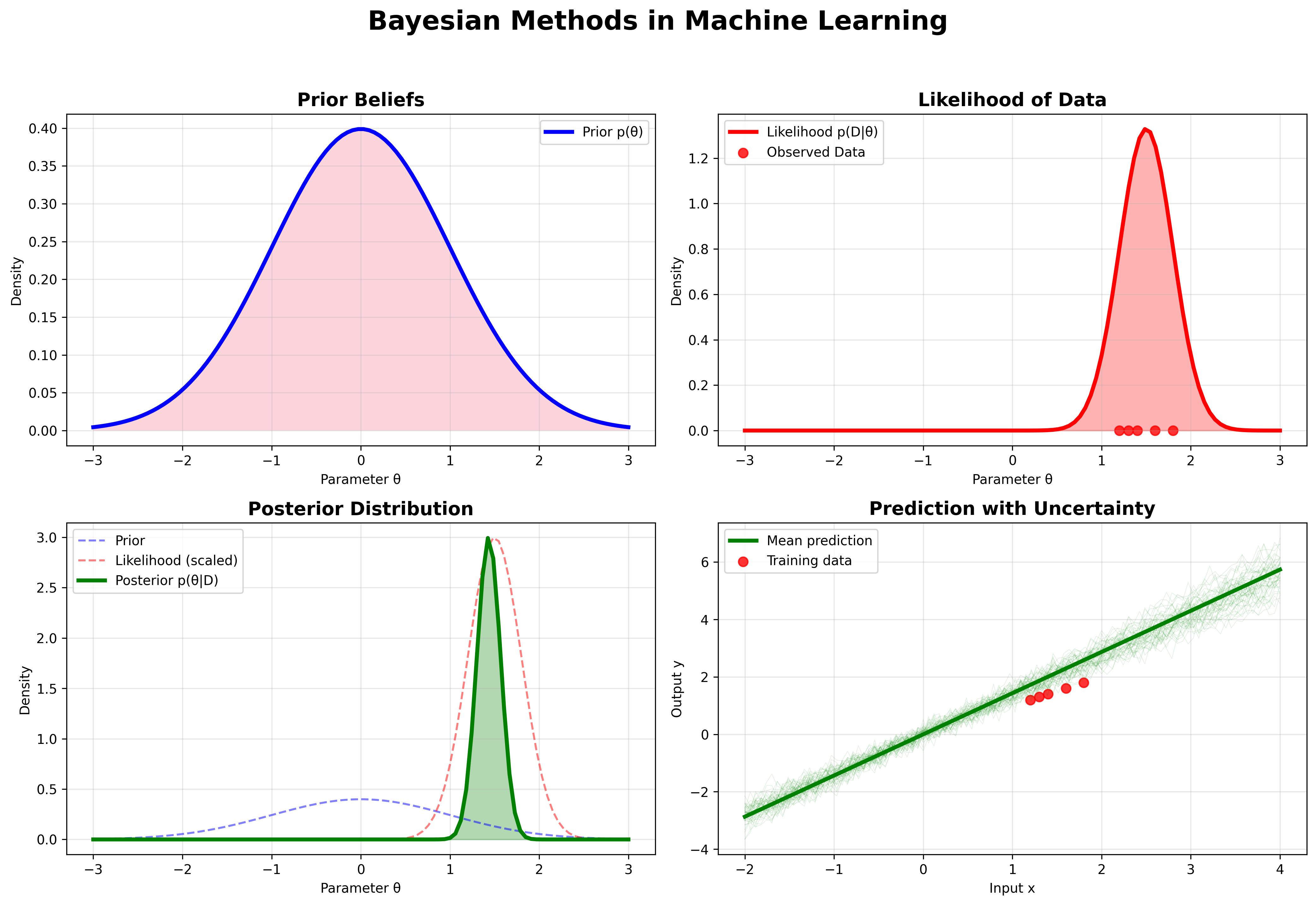
Bayesian methods provide a principled framework for handling uncertainty in machine learning. Unlike frequentist approaches that treat model parameters as fixed but unknown values, Bayesian methods treat parameters as random variables with probability distributions. This fundamental shift in perspective leads to more robust, interpretable, and uncertainty-aware machine learning models.
Figure 1: Bayesian methods provide a principled approach to uncertainty quantification in machine learning.
Table of Contents
- Foundations of Bayesian Thinking
- Bayes' Theorem in Machine Learning
- Bayesian Linear Regression
- Bayesian Neural Networks
- Markov Chain Monte Carlo (MCMC)
- Variational Inference
- Applications and Case Studies
- Implementation Examples
- Advantages and Challenges
- Future Directions
Foundations of Bayesian Thinking {#foundations}
The Bayesian Paradigm
The core of Bayesian thinking lies in the systematic updating of beliefs based on evidence. In machine learning, this translates to:
- Prior Knowledge: What we believe about model parameters before seeing data
- Likelihood: How well our model explains the observed data
- Posterior: Updated beliefs after incorporating the evidence
Key Concepts
Prior Distribution : Represents our initial beliefs about parameter before observing data.
Likelihood : The probability of observing data given parameter .
Posterior Distribution : Our updated beliefs about after observing data .
Evidence : The marginal likelihood, often used for model comparison.
Bayes' Theorem in Machine Learning {#bayes-theorem}
The foundation of all Bayesian methods is Bayes' theorem:
Where:
- is the posterior distribution
- is the likelihood
- is the prior distribution
- is the evidence
Predictive Distribution
For making predictions on new data , we use the posterior predictive distribution:
This integral over all possible parameter values naturally incorporates model uncertainty into predictions.
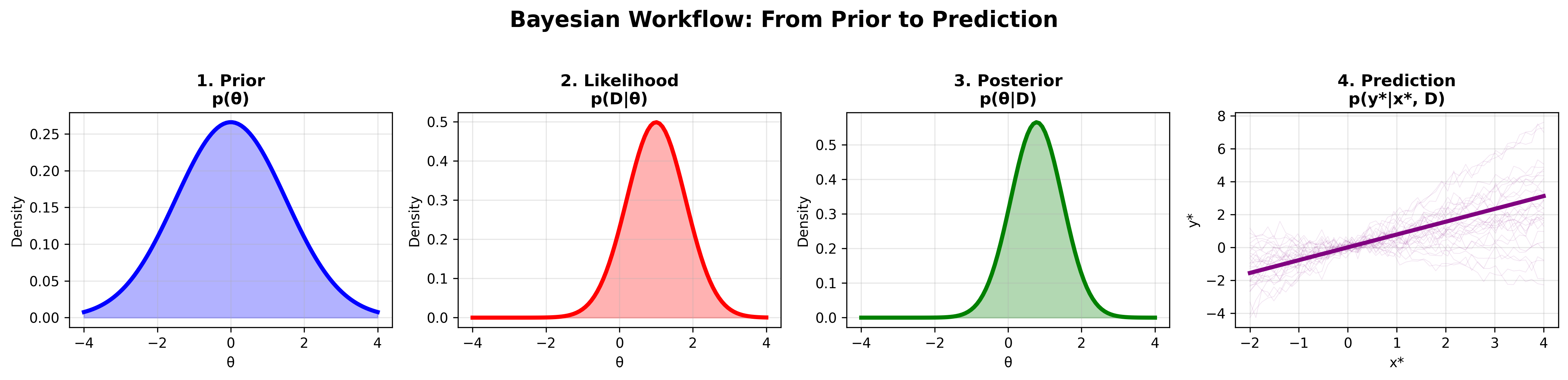 Figure 2: The Bayesian workflow showing the progression from prior to posterior through likelihood.
Bayesian Linear Regression {#bayesian-regression}
Let's start with the simplest case: Bayesian linear regression. Unlike ordinary least squares, which finds point estimates of parameters, Bayesian linear regression maintains full distributions over parameters.
Model Setup
Consider the linear regression model:
where .
Prior Specification
We place priors on the parameters:
Posterior Inference
With conjugate priors, the posterior distributions have closed-form solutions:
where:
Advantages
- Uncertainty Quantification: Natural confidence intervals for predictions
- Regularization: Prior acts as regularizer, preventing overfitting
- Model Selection: Automatic relevance determination through hierarchical priors
Bayesian Neural Networks {#bayesian-neural-networks}
Extending Bayesian principles to neural networks creates models that can express uncertainty about their predictions—crucial for safety-critical applications.
Weight Uncertainty
Instead of point estimates for weights , we maintain distributions:
Prediction with Uncertainty
For a new input , predictions integrate over all possible weight configurations:
Practical Approximations
Since exact inference is intractable, we use approximations:
- Variational Inference: Approximate posterior with tractable distribution
- Monte Carlo Dropout: Use dropout at test time to approximate uncertainty
- Ensemble Methods: Train multiple networks and average predictions
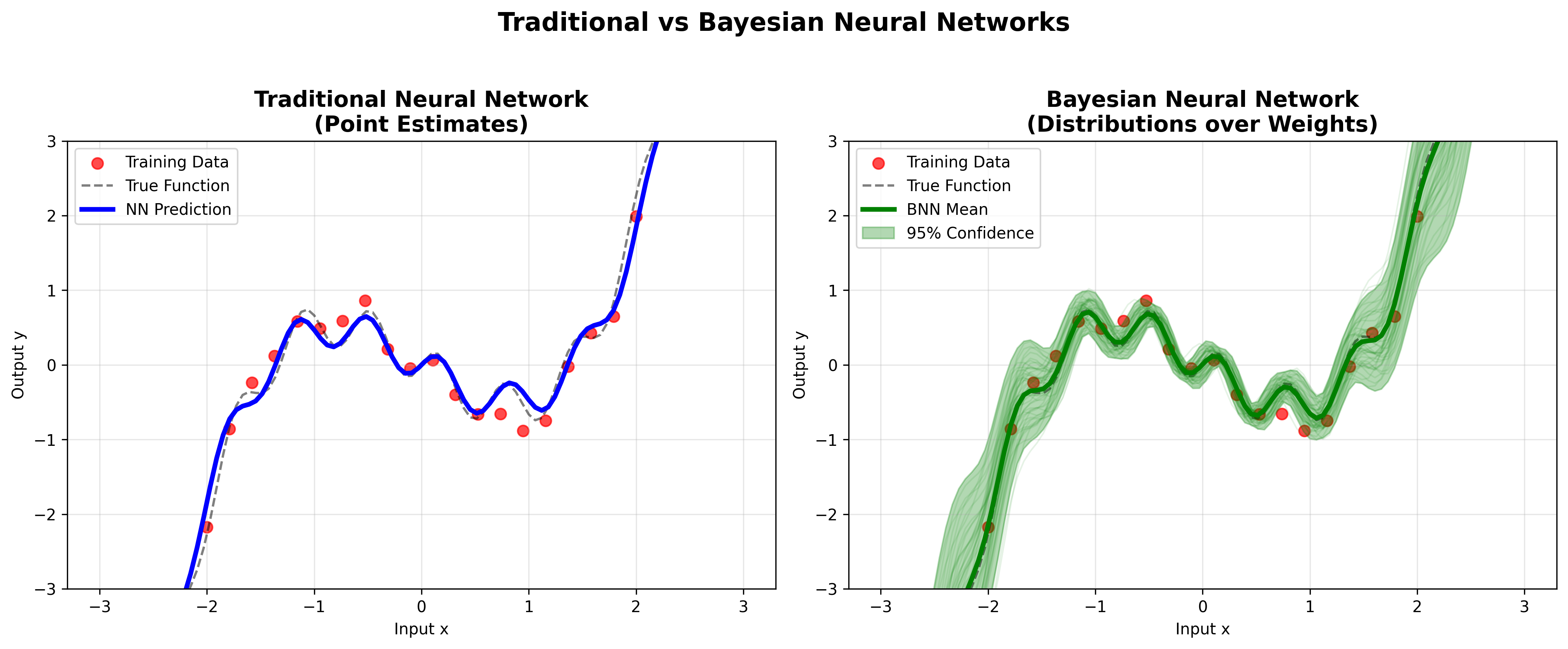 Figure 3: Comparison of traditional neural networks (point estimates) vs. Bayesian neural networks (distributions).
Markov Chain Monte Carlo (MCMC) {#mcmc}
When posterior distributions don't have closed-form solutions, MCMC methods provide a way to sample from complex distributions.
The MCMC Framework
MCMC constructs a Markov chain whose stationary distribution is the target posterior .
Popular MCMC Algorithms
Metropolis-Hastings Algorithm:
- Propose new state from proposal distribution
- Calculate acceptance probability:
- Accept with probability
Hamiltonian Monte Carlo (HMC): Uses gradient information to make efficient proposals in high-dimensional spaces.
No-U-Turn Sampler (NUTS): Automatically tunes HMC step size and number of steps.
Convergence Diagnostics
- Trace Plots: Visual inspection of chain mixing
- Gelman-Rubin Statistic: Compares within-chain and between-chain variance
- Effective Sample Size: Accounts for autocorrelation in samples
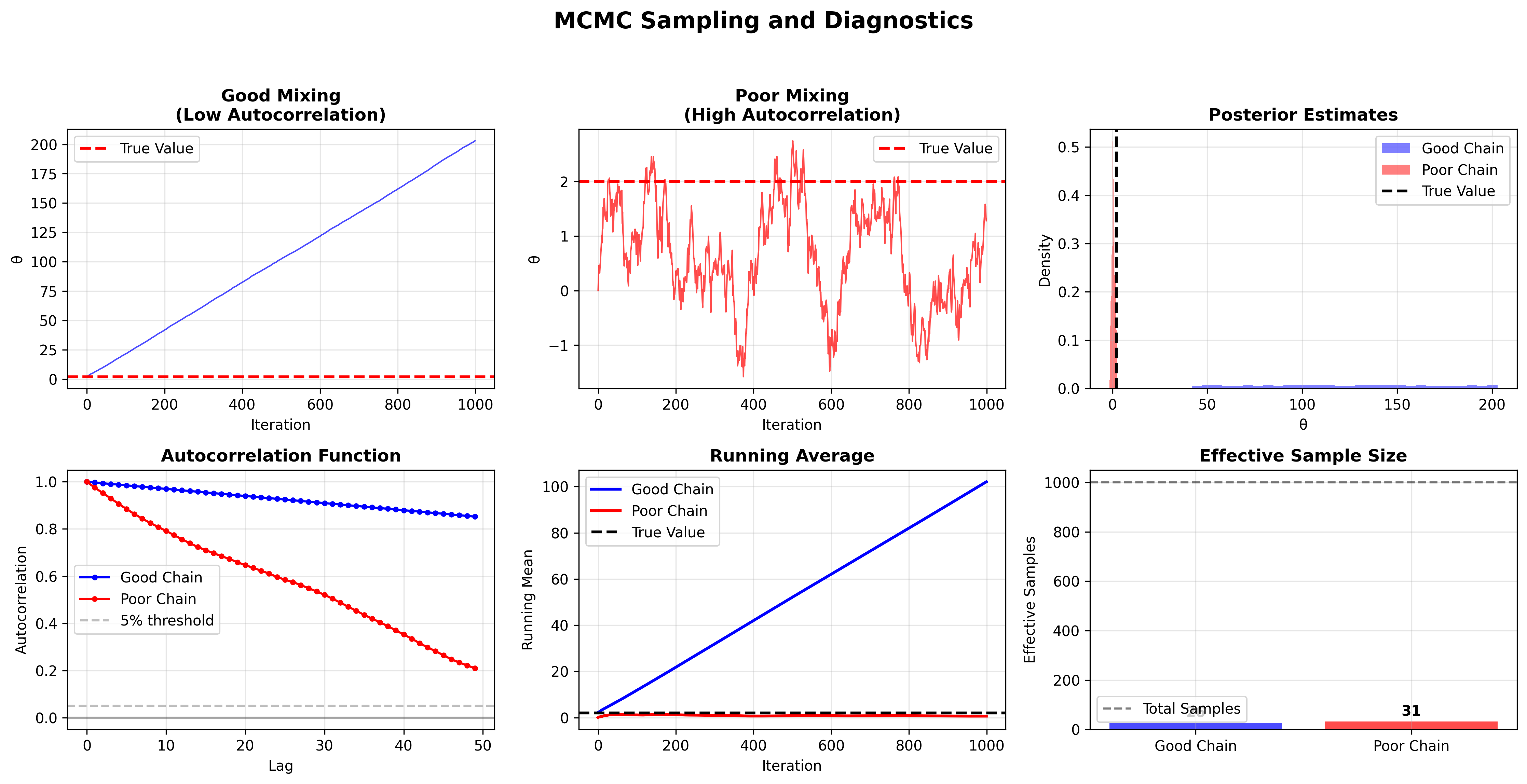 Figure 5: MCMC sampling diagnostics showing the difference between well-mixed and poorly-mixed chains.
Variational Inference {#variational-inference}
Variational inference approximates intractable posteriors with tractable distributions by solving an optimization problem.
The Variational Objective
We choose a family of distributions and find the member that minimizes the KL divergence:
This is equivalent to maximizing the Evidence Lower Bound (ELBO):
Mean Field Approximation
A common choice is the mean field approximation:
This assumes independence between parameters, making optimization tractable.
Stochastic Variational Inference
For large datasets, we can use stochastic optimization:
- Sample mini-batch of data
- Compute noisy gradient of ELBO
- Update variational parameters using stochastic gradient ascent
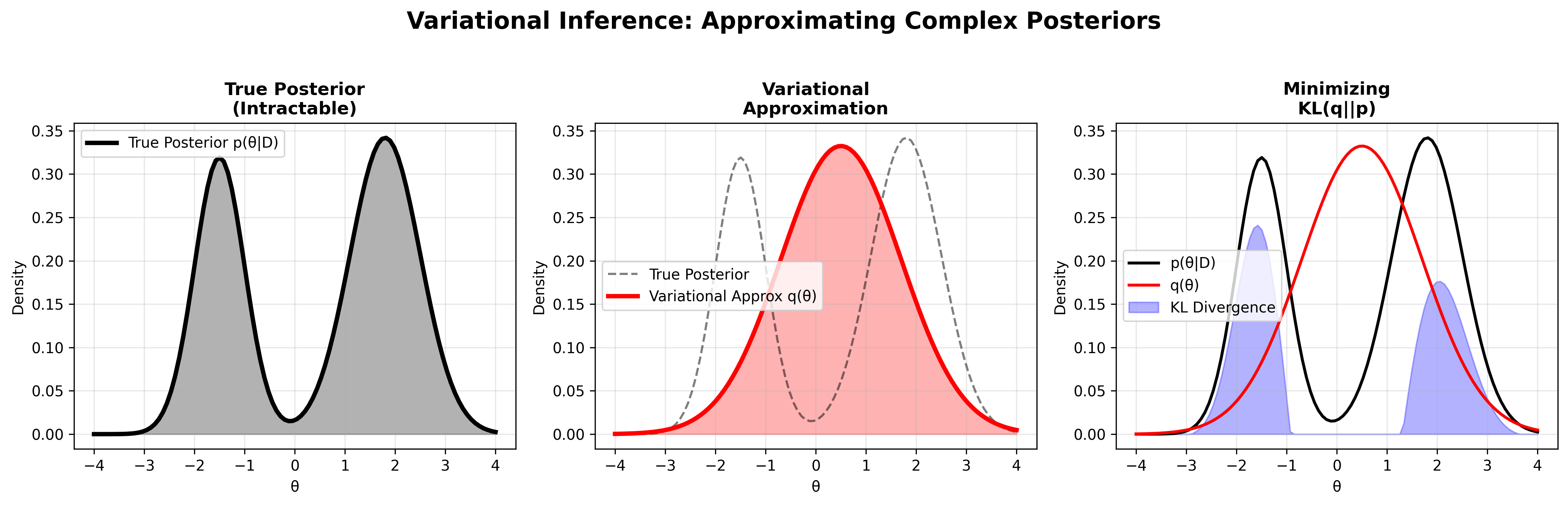 Figure 4: Variational inference approximates the true posterior with a simpler distribution.
Applications and Case Studies {#applications}
1. Bayesian Optimization
Bayesian optimization uses Gaussian processes to model objective functions and acquisition functions to guide search:
Applications:
- Hyperparameter tuning
- Neural architecture search
- Drug discovery
- Materials design
2. Bayesian Deep Learning
Uncertainty Types:
- Aleatoric: Data inherent uncertainty
- Epistemic: Model uncertainty due to limited data
Applications:
- Medical diagnosis
- Autonomous driving
- Financial modeling
- Scientific discovery
3. Bayesian Nonparametrics
Models that can grow in complexity with data:
- Dirichlet Process: Infinite mixture models
- Gaussian Process: Flexible function approximation
- Indian Buffet Process: Infinite feature models
4. Online Learning
Bayesian methods naturally handle streaming data:
Implementation Examples {#implementation}
Bayesian Linear Regression in Python
import numpy as np
import scipy.stats as stats
import matplotlib.pyplot as plt

class BayesianLinearRegression:
    def __init__(self, alpha=1.0, beta=1.0):
        self.alpha = alpha  # Precision of prior
        self.beta = beta    # Precision of noise

    def fit(self, X, y):
        # Add bias term
        X = np.column_stack([np.ones(X.shape[0]), X])

        # Prior parameters
        S0_inv = self.alpha * np.eye(X.shape[1])
        m0 = np.zeros(X.shape[1])

        # Posterior parameters
        SN_inv = S0_inv + self.beta * X.T @ X
        self.SN = np.linalg.inv(SN_inv)
        self.mN = self.SN @ (S0_inv @ m0 + self.beta * X.T @ y)

        self.X_train = X
        self.y_train = y

    def predict(self, X_test, return_std=False):
        X_test = np.column_stack([np.ones(X_test.shape[0]), X_test])

        # Predictive mean
        y_mean = X_test @ self.mN

        if return_std:
            # Predictive variance
            y_var = 1/self.beta + np.diag(X_test @ self.SN @ X_test.T)
            y_std = np.sqrt(y_var)
            return y_mean, y_std

        return y_mean
Complete Working Example
You can find a complete, runnable implementation of Bayesian Linear Regression here. This example includes:
- Full Bayesian linear regression class
- Uncertainty quantification
- Posterior visualization
- Interactive demo with synthetic data
Bayesian Neural Network with Variational Inference```
Bayesian Neural Network with Variational Inference
import torch
import torch.nn as nn
import torch.nn.functional as F
from torch.distributions import Normal

class BayesianLinear(nn.Module):
    def __init__(self, in_features, out_features):
        super().__init__()

        # Weight parameters
        self.weight_mu = nn.Parameter(torch.randn(out_features, in_features))
        self.weight_rho = nn.Parameter(torch.randn(out_features, in_features))

        # Bias parameters
        self.bias_mu = nn.Parameter(torch.randn(out_features))
        self.bias_rho = nn.Parameter(torch.randn(out_features))

    def forward(self, x):
        # Sample weights and biases
        weight_sigma = torch.log(1 + torch.exp(self.weight_rho))
        weight = Normal(self.weight_mu, weight_sigma).rsample()

        bias_sigma = torch.log(1 + torch.exp(self.bias_rho))
        bias = Normal(self.bias_mu, bias_sigma).rsample()

        return F.linear(x, weight, bias)

class BayesianNN(nn.Module):
    def __init__(self, input_dim, hidden_dim, output_dim):
        super().__init__()
        self.layer1 = BayesianLinear(input_dim, hidden_dim)
        self.layer2 = BayesianLinear(hidden_dim, output_dim)

    def forward(self, x):
        x = torch.relu(self.layer1(x))
        return self.layer2(x)
Advantages and Challenges {#pros-cons}
Advantages
-
Principled Uncertainty Quantification
- Natural measure of confidence in predictions
- Distinguishes between different types of uncertainty
-
Automatic Model Selection
- Occam's razor built into framework
- No need for separate validation procedures
-
Robust to Overfitting
- Prior regularization prevents extreme parameter values
- Model averaging reduces variance
-
Interpretability
- Clear probabilistic interpretation of results
- Transparent handling of assumptions
Challenges
-
Computational Complexity
- Posterior inference often intractable
- Approximation methods required
-
Prior Specification
- Choice of prior can significantly impact results
- Difficulty in encoding domain knowledge
-
Scalability
- MCMC methods can be slow for large datasets
- Memory requirements for storing samples
-
Implementation Complexity
- More complex than point estimation methods
- Requires understanding of probability theory
Future Directions {#future}
Scalable Bayesian Methods
- Stochastic Variational Inference: Handling massive datasets
- Distributed MCMC: Parallel sampling strategies
- Gaussian Process Approximations: Sparse methods for large-scale GP inference
Deep Bayesian Learning
- Bayesian Transformers: Uncertainty in attention mechanisms
- Bayesian Reinforcement Learning: Safe exploration strategies
- Bayesian Generative Models: Uncertainty in VAEs and GANs
Automated Bayesian Modeling
- Probabilistic Programming: Languages like Stan, PyMC, Pyro
- Automated Prior Selection: Data-driven prior specification
- Model Discovery: Automatic structure learning
Applications in AI Safety
- Uncertainty-Aware Decision Making: Critical for autonomous systems
- Out-of-Distribution Detection: Identifying when models are uncertain
- Calibrated Predictions: Ensuring predicted probabilities are meaningful
Conclusion
Bayesian methods provide a powerful and principled framework for machine learning that naturally handles uncertainty and incorporates prior knowledge. While computational challenges remain, recent advances in variational inference, MCMC methods, and probabilistic programming have made Bayesian machine learning increasingly practical.
The key insight of Bayesian methods—treating model parameters as random variables rather than fixed values—leads to more robust, interpretable, and uncertainty-aware models. As machine learning systems are deployed in increasingly critical applications, the ability to quantify and reason about uncertainty becomes essential.
Whether you're working on medical diagnosis, autonomous vehicles, or financial modeling, understanding Bayesian methods will make you a more effective machine learning practitioner. The investment in learning these concepts pays dividends in building more reliable and trustworthy AI systems.
Further Reading
-
Books:
- "Pattern Recognition and Machine Learning" by Christopher Bishop
- "Bayesian Reasoning and Machine Learning" by David Barber
- "Machine Learning: A Probabilistic Perspective" by Kevin Murphy
-
Papers:
- "Weight Uncertainty in Neural Networks" (Blundell et al., 2015)
- "Variational Inference: A Review for Statisticians" (Blei et al., 2017)
- "Bayesian Deep Learning" (Wang & Yeung, 2016)
-
Software:
- PyMC: Probabilistic programming in Python
- Stan: Platform for statistical modeling
- Pyro: Deep universal probabilistic programming
This post provides a comprehensive introduction to Bayesian methods in machine learning. For more advanced topics and practical implementations, check out our other posts on Gaussian Processes and Mathematical Foundations of ML.
Related Posts
More content from the Machine Learning category and similar topics
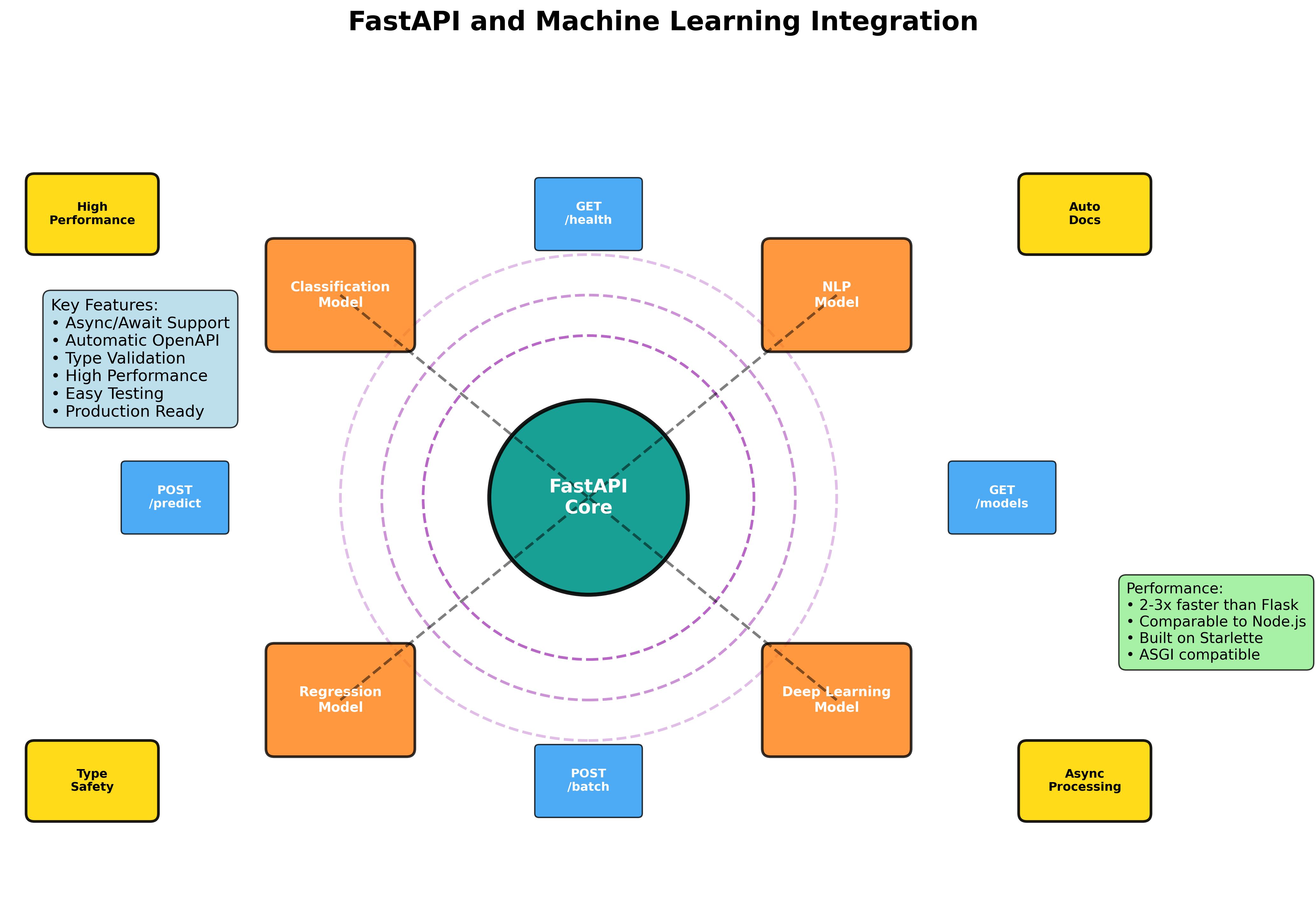
Master the art of building production-ready machine learning APIs with FastAPI. From basic model serving to advanced async processing and containerized deployment.
Shared topics:
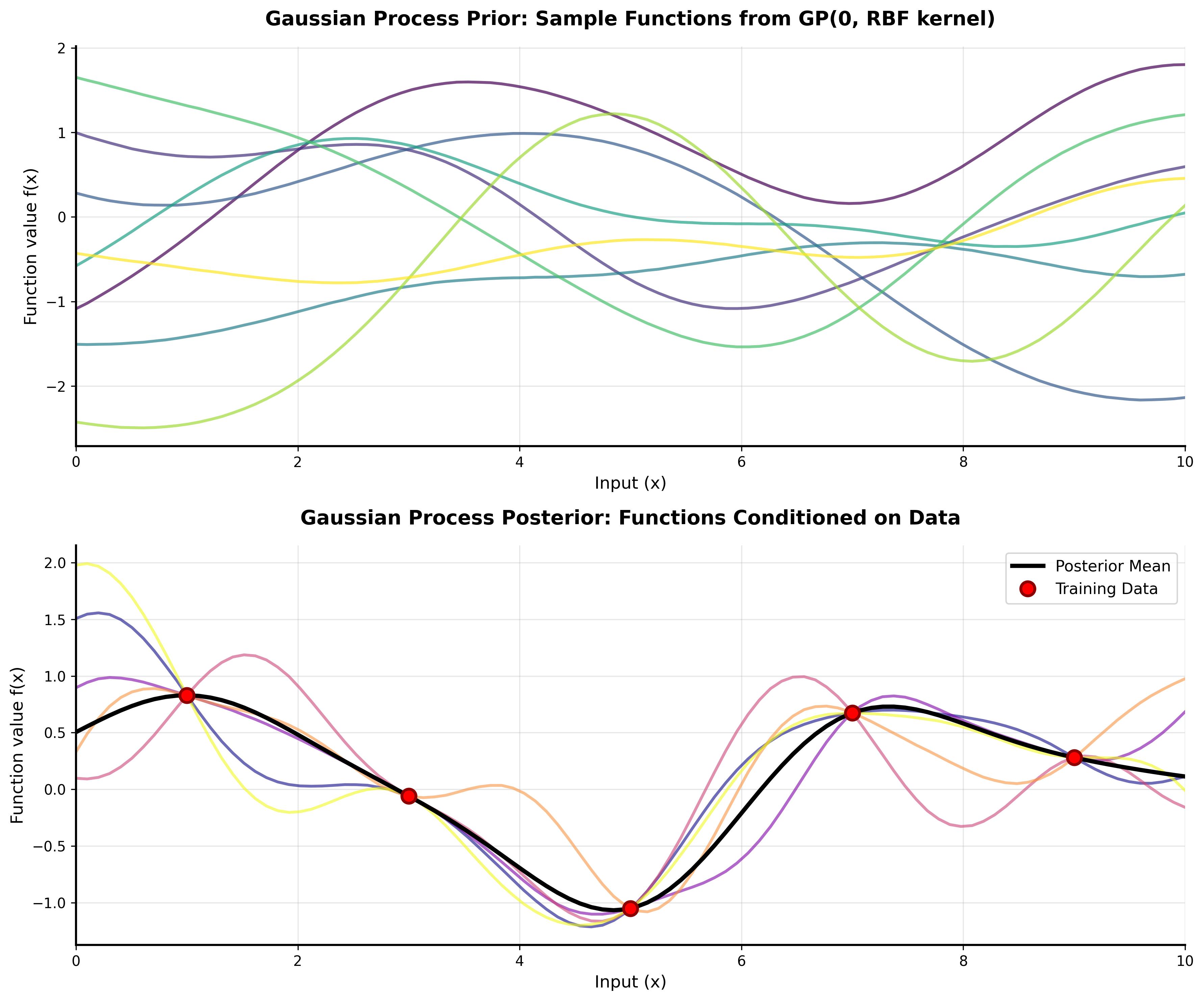
A comprehensive tutorial on understanding Gaussian Processes with interactive visualizations and practical examples.

A comprehensive tutorial on understanding Gaussian Processes with interactive visualizations and practical examples.