Introduction to Functional Data Analysis with R

Functional Data Analysis (FDA) is a fascinating branch of statistics that treats data as functions rather than discrete observations. Instead of analyzing individual data points, we analyze entire curves, surfaces, or other functional objects.

What is Functional Data Analysis?

Imagine you're studying temperature patterns throughout the day across different cities. Traditional analysis might look at temperature at specific times (8 AM, 12 PM, 6 PM). FDA, however, treats the entire temperature curve as a single observation—a function that maps time to temperature.

This perspective is powerful because:

It preserves the continuity and smoothness of the underlying process
It can handle irregularly spaced observations
It naturally incorporates the functional nature of many real-world phenomena

Key Concepts

1. Functional Objects

In FDA, our data consists of functions $x_i(t)$ where:

$i = 1, 2, ..., n$ indexes the different functional observations
$t$ is the argument (time, space, frequency, etc.)
Each $x_i(t)$ is a complete function, not just a set of points

2. Basis Function Representation

Since we can't work with infinite-dimensional functions directly, we represent them using basis functions:

$x_i(t) = \sum_{k=1}^K c_{ik} \phi_k(t)$

Where:

$\phi_k(t)$ are basis functions (B-splines, Fourier, wavelets, etc.)
$c_{ik}$ are coefficients
$K$ is the number of basis functions

3. Smoothing

Real data is often noisy, so we need to smooth our functional observations:

$\min_{x} \int [y_i(t_j) - x_i(t_j)]^2 dt + \lambda \int [D^m x_i(t)]^2 dt$

The first term ensures fidelity to data, the second term (with roughness penalty $\lambda$ ) ensures smoothness.

Getting Started with R

Let's dive into implementation using R's powerful FDA ecosystem:

# Load essential libraries
library(fda)
library(ggplot2)
library(dplyr)
library(tidyr)

# Set up for reproducibility
set.seed(123)

Creating Functional Data Objects

# Generate sample data: daily temperature curves for 30 days
n_days <- 30
time_points <- seq(0, 24, length.out = 25)  # Hours 0-24

# Generate temperature data with daily patterns
temperature_data <- matrix(NA, nrow = n_days, ncol = length(time_points))

for (i in 1:n_days) {
  # Base temperature pattern: cool at night, warm during day
  base_temp <- 15 + 10 * sin(2 * pi * (time_points - 6) / 24)
  
  # Add daily variation and noise
  daily_effect <- rnorm(1, 0, 3)
  noise <- rnorm(length(time_points), 0, 1)
  
  temperature_data[i, ] <- base_temp + daily_effect + noise
}

# Create B-spline basis
n_basis <- 15
temp_basis <- create.bspline.basis(rangeval = c(0, 24), 
                                   nbasis = n_basis, 
                                   norder = 4)

# Convert data to functional data object
temp_fd <- Data2fd(argvals = time_points,
                   y = t(temperature_data),
                   basisobj = temp_basis)

print(temp_fd)

Visualizing Functional Data

# Plot the functional data
plot(temp_fd, 
     main = "Daily Temperature Curves",
     xlab = "Hour of Day", 
     ylab = "Temperature (°C)",
     col = rainbow(n_days),
     lty = 1)

# Add mean curve
mean_temp <- mean.fd(temp_fd)
lines(mean_temp, lwd = 3, col = "black")
legend("topright", legend = c("Individual days", "Mean"), 
       col = c("rainbow", "black"), lwd = c(1, 3))

Functional Principal Component Analysis

FPCA is the functional analog of PCA, helping us understand the main modes of variation:

# Perform FPCA
temp_pca <- pca.fd(temp_fd, nharm = 4)

# Print variance explained
print(temp_pca$varprop)

# Plot the principal components
par(mfrow = c(2, 2))
for (i in 1:4) {
  plot(temp_pca$harmonics[i], 
       main = paste("PC", i, "- Variance:", 
                   round(temp_pca$varprop[i] * 100, 1), "%"),
       xlab = "Hour", ylab = "PC Loading")
}

Understanding the components:

PC1: Often captures overall level differences (some days warmer than others)
PC2: Might capture timing differences (peak temperature earlier/later)
PC3 & 4: More subtle variations in curve shape

Functional Regression

Let's predict maximum daily temperature from the functional curves:

# Create response variable: maximum temperature each day
max_temps <- apply(eval.fd(time_points, temp_fd), 2, max)

# Functional linear regression
temp_reg <- fRegress(max_temps ~ temp_fd)

# Print results
print(temp_reg$betaestlist)

# Plot the regression coefficient function
plot(temp_reg$betaestlist$temp_fd$fd,
     main = "Regression Coefficient Function",
     xlab = "Hour of Day",
     ylab = "Coefficient")

The coefficient function tells us how temperature at each hour contributes to predicting the daily maximum.

Advanced Topics

1. Functional ANOVA

# Simulate data with group differences
group_A <- temp_fd[1:15]  # First 15 days
group_B <- temp_fd[16:30] # Last 15 days

# Add systematic difference to group B
group_B_adjusted <- group_B + 5  # 5°C warmer

# Combine for ANOVA
combined_fd <- c(group_A, group_B_adjusted)
groups <- factor(rep(c("A", "B"), each = 15))

# Functional ANOVA
fanova_result <- fanova.tests(combined_fd, groups)
print(fanova_result)

2. Derivative Analysis

Derivatives reveal important features like rates of change:

# Compute first derivative (rate of temperature change)
temp_deriv1 <- deriv.fd(temp_fd, 1)

# Plot derivatives
plot(temp_deriv1,
     main = "Temperature Rate of Change",
     xlab = "Hour of Day",
     ylab = "°C per Hour",
     col = rainbow(n_days))

# Find times of maximum heating/cooling
mean_deriv <- mean.fd(temp_deriv1)
deriv_vals <- eval.fd(time_points, mean_deriv)
max_heating_time <- time_points[which.max(deriv_vals)]
max_cooling_time <- time_points[which.min(deriv_vals)]

cat("Maximum heating around:", max_heating_time, "hours\n")
cat("Maximum cooling around:", max_cooling_time, "hours\n")

3. Functional Clustering

# Distance-based clustering of functional data
# Compute L2 distances between curves
dist_matrix <- matrix(NA, n_days, n_days)

for (i in 1:n_days) {
  for (j in 1:n_days) {
    diff_fd <- temp_fd[i] - temp_fd[j]
    dist_matrix[i, j] <- sqrt(inprod(diff_fd, diff_fd))
  }
}

# Hierarchical clustering
hc_result <- hclust(as.dist(dist_matrix), method = "ward.D2")

# Plot dendrogram
plot(hc_result, main = "Functional Data Clustering")

# Get clusters
clusters <- cutree(hc_result, k = 3)

# Visualize clusters
plot(temp_fd, col = clusters, main = "Temperature Clusters")

Real-World Applications

1. Growth Curves in Biology

# Simulate growth data
ages <- seq(0, 18, length.out = 20)
n_children <- 50

growth_data <- matrix(NA, n_children, length(ages))
for (i in 1:n_children) {
  # Logistic growth with individual variation
  max_height <- rnorm(1, 170, 10)
  growth_rate <- rnorm(1, 0.8, 0.1)
  inflection <- rnorm(1, 12, 1)
  
  growth_data[i, ] <- max_height / (1 + exp(-growth_rate * (ages - inflection)))
}

# Create functional data object
growth_basis <- create.bspline.basis(c(0, 18), nbasis = 12, norder = 4)
growth_fd <- Data2fd(ages, t(growth_data), growth_basis)

# Analyze growth velocity (first derivative)
velocity_fd <- deriv.fd(growth_fd, 1)
plot(velocity_fd, main = "Growth Velocity Curves", 
     xlab = "Age", ylab = "Height Velocity (cm/year)")

2. Financial Time Series

# Simulate daily return curves
trading_hours <- seq(9, 17, length.out = 50)  # 9 AM to 5 PM
n_trading_days <- 100

returns_data <- matrix(NA, n_trading_days, length(trading_hours))
for (i in 1:n_trading_days) {
  # Random walk with intraday patterns
  volatility_pattern <- 0.5 + 0.3 * sin(2 * pi * (trading_hours - 9) / 8)
  returns_data[i, ] <- cumsum(rnorm(length(trading_hours), 0, volatility_pattern))
}

# Functional analysis of returns
returns_basis <- create.fourier.basis(c(9, 17), nbasis = 21)
returns_fd <- Data2fd(trading_hours, t(returns_data), returns_basis)

# Analyze volatility patterns
volatility_fd <- deriv.fd(returns_fd, 1)^2  # Squared derivative as volatility proxy
mean_volatility <- mean.fd(volatility_fd)

plot(mean_volatility, main = "Average Intraday Volatility Pattern",
     xlab = "Trading Hour", ylab = "Volatility")

Best Practices and Tips

1. Choosing Basis Functions

B-splines: Good general choice, flexible, local support
Fourier: Perfect for periodic data
Wavelets: Good for data with local features
Polynomials: Simple but can be unstable

2. Selecting Number of Basis Functions

# Cross-validation for basis selection
gcv_scores <- numeric(20)

for (k in 5:25) {
  basis_k <- create.bspline.basis(c(0, 24), nbasis = k, norder = 4)
  fd_k <- Data2fd(time_points, t(temperature_data), basis_k, lambda = 1e-6)
  gcv_scores[k-4] <- mean(fd_k$gcv)
}

optimal_k <- which.min(gcv_scores) + 4
cat("Optimal number of basis functions:", optimal_k, "\n")

3. Handling Missing Data

# Simulate data with missing observations
temp_data_missing <- temperature_data
temp_data_missing[sample(length(temp_data_missing), 
                        length(temp_data_missing) * 0.1)] <- NA

# FDA can handle missing data naturally
temp_fd_missing <- Data2fd(time_points, t(temp_data_missing), temp_basis)

# The functional representation interpolates missing values
plot(temp_fd_missing[1:5], main = "Functional Data with Missing Observations")

Conclusion

Functional Data Analysis opens up new perspectives on data that naturally exists as functions. By treating curves, surfaces, and other functional objects as single entities, FDA provides:

More natural representations of continuous processes
Powerful tools for understanding functional variation
Robust methods for prediction and classification
Elegant handling of irregular and missing data

The R ecosystem for FDA is mature and comprehensive, with the fda package providing most essential tools. As you dive deeper, you'll find FDA particularly valuable for:

Longitudinal studies in biology and medicine
Environmental monitoring data
Economic and financial time series
Signal processing and image analysis
Any domain where the functional nature of data matters

FDA represents a fundamental shift in thinking—from points to functions, from discrete to continuous, from fragmented to holistic. Once you start seeing your data as functions, you'll discover new insights and possibilities.

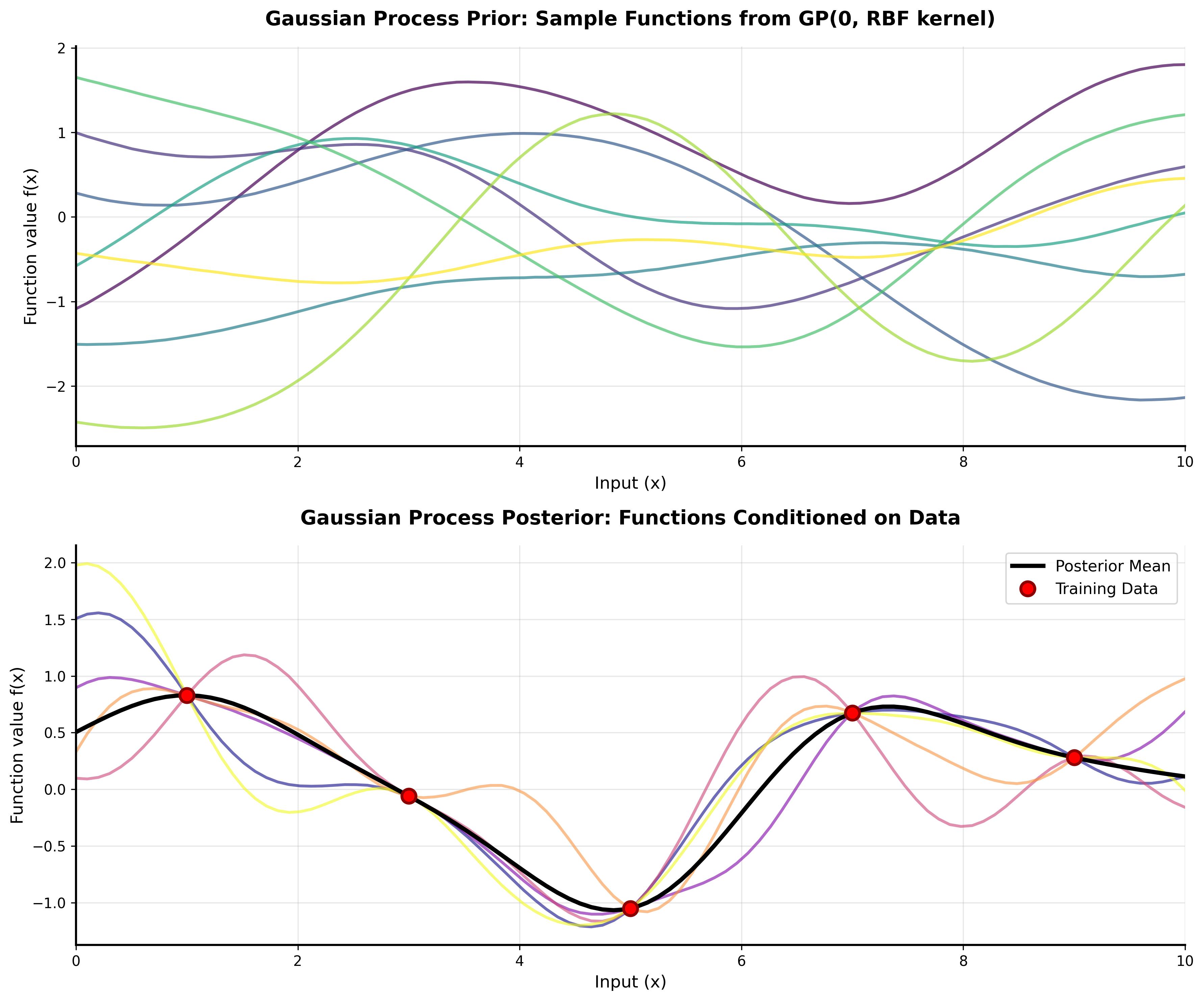
Interested in the mathematical details? Check out my post on Gaussian Processes for related functional modeling techniques.

Introduction to Functional Data Analysis with R

Introduction to Functional Data Analysis with R

What is Functional Data Analysis?

Key Concepts

1. Functional Objects

2. Basis Function Representation

3. Smoothing

Getting Started with R

Creating Functional Data Objects

Visualizing Functional Data

Functional Principal Component Analysis

Functional Regression

Advanced Topics

1. Functional ANOVA

2. Derivative Analysis

3. Functional Clustering

Real-World Applications

1. Growth Curves in Biology

2. Financial Time Series

Best Practices and Tips

1. Choosing Basis Functions

2. Selecting Number of Basis Functions

3. Handling Missing Data

Conclusion

Related Posts

Comments & Discussion

Share this post